Forecasting Using Prior Distributions

We have been building some product forecasting models using Monte Carlo methods. Sales distributions are often skewed right. Using normal approximations tends to over inflate forecast estimates, since the distribution is not centered around the mean. Further more the standard deviation of skewed distributions tends to produce estimates with very wide variances - by definition.

To overcome this, we use a Monte Carlo simulator - that draws from the sales distribution at random. Creating a sample of many estimates not only gives a more accurate estimate, it is also helps us calculate more realistic margins of error.

Fast Tracking Data Analysis

Not all variables in a data set or questions in a survey are equal when it comes to data analysis and analytics. Some variables (questions if it’s a survey) will be inherently better at classifying outcomes than others. For example, if you are using a data set to build a narrative around a particular binary behavior (i.e. people who do X vs people who don't do X) then there are some considerations about which variables will give you a short cut to the story.

The first rule of thumb is to start with binary predictors, i.e. variables with only two different responses / values. Variables with a greater number of possible responses/values will be more likely to have spurious relationships with the variable that you are trying to predict. Predictors with two levels are less likely to suffer this phenomena.

The second rule of thumb is to select those binary variables that have a similar distribution to the variable that you are trying to predict. For example if you are trying to predict a behavior that has 20% incidence among a certain population then the best predictors to use should also have a 20% / 80% spread across two values.

The reason for this condition being optimal is easily explained. The best predictor is one that identifies all cases correctly. Imagine that the best predictor has two possible values with 40% of cases at a value of 1 and 60% of the cases have a value of 2 in this variable. With this distribution, if 1s are predictive of the behavior we are modelling then only half the 1s can be correctly predictive if the behavior has a 20% incidence. The other half of the 1s are incorrectly predictive.  However, if the best predictor had 15% of cases that were 1s and 85% cases had a value of 2 then all the 1s could be correctly predictive. This would be a much better predictor to use - in part because the incidence of 1s (or 2s for that matter) is close to the incidence of behavior we are predicting - meaning that 1s have a better chance of being better predictors.

I have a nice graph to show this too. Watch this space!

Random Forests and The Power of Guessing for Low Incidence Features

We have been thinking a lot about the relationship between the incidence of the feature we are trying to predict and the usefulness of analytics algorithms. In previous posts (here and here) we looked at the guessing the feature rather than using an analytics model. When the incidence of the feature you are trying to predict is low, it is sometimes worth guessing than running an analytics algorithm since the accuracy will be higher for low incidence features.

If you then consider how Random Forests work (create a family of decision trees at random ->  use the modal value predicted by the family as the correctly classified answer), it becomes clear that these are just a mechanism for creating lots of guesses and when the incidence is low, a guess is better than an analytical prediction. Obviously, this isn't to undermine Random Forests, more an observation as to perhaps why they work so well.

We have never really looked at the efficiency of the KL algorithm vs a straight guess as we work down further into a decision tree. However,  what we have incorporated is a means of more efficient deployment of resources (servers and processors).  The latest release of the product allows users to set a stopping criteria based on the incidence of the predicted feature for a particular branch in the learning tree. As we have seen (here) , incidence levels effect the point at which the user is better off making a guess than relying on an analytics algorithm. The stopping criteria prevents the application going past the point at which a guess would be better.


Simple Accuracy Calculator

I used the accuracy calculation equation to make this simple form that works out how well a prediction must perform to be better than a weighted guess. For example if the incidence of what we are trying to predict is 40% (gender=female, for example) then the model prediction must have an accuracy greater than 52% for it to be better than randomly assigning 40% of cases to gender is female  and assigning the other 60% to gender isn't female. As this weighted-guess will have an accuracy of 52% over a large sample.

When It Comes To Rules Based Classification, Less Is More

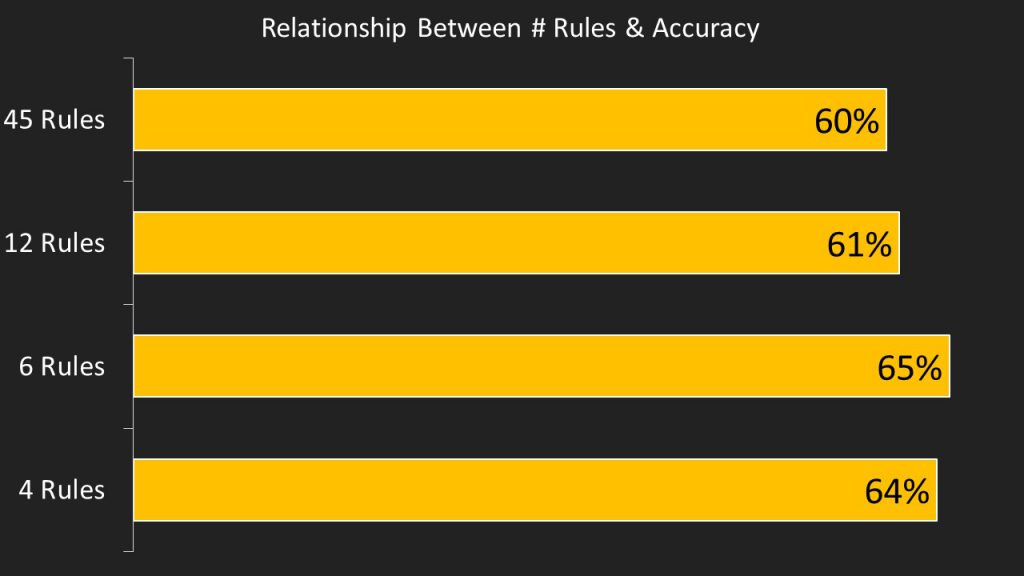
We have been running trials on a 16 question survey, predicting the responses to a particular question using other data in the survey. What we discovered is that the more rules we allowed KL analytics engine to produce, the lower the accuracy and the harder it becomes to explain the model to another person.

Predictive Accuracy of Knowledge Leaps Analytics Engine Using 10-Fold Validation - Best Guess Accuracy = 50.2%


Knowing When to Guess

When it comes to designing and implementing algorithms for Knowledge Leaps I have spent a lot of time thinking about accuracy in relation to making predictions. I soon realized that there is a mathematical relationship between the accuracy of a guess and the incidence of what you are trying to predict.

For instance, if you have built a model for predicting whether or not a roulette ball will fall into the zero slot on a roulette wheel with 37 numbers (0-36) then your model has to be correct (at predicting success or failure) at least 94.67% of the time.  However, if you want to predict red or black then your model needs to be correct 50.04% of the time to be better than a pure guess.

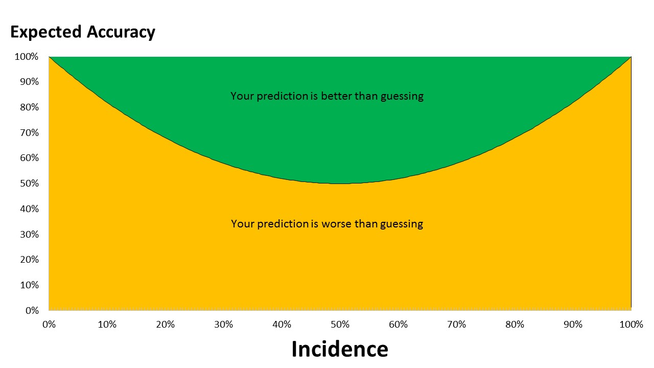
The graph below shows the relationship as a function of incidence (the rate of what we are trying to predict).

Broad conclusions we can draw from this relationship:

  • When we are trying to predict outcomes which have an incidence of between 20% and 80%, there is a lot of potential for producing a worthwhile model that can improve on a guess.
  • When the incidence of outcomes is less than 5% and greater than 95%, models need to be delivering 91%+ accuracy to be of any help. This is the realm of medical diagnosis, an area where guesswork isn't welcome.
  • Since 66% of the chart is territory where a guess is better than a model, if we produced random models to make a prediction, 66% of the time a guess would be better. Obviously, if we aggregate up the results of lots of random guesses we can produce more accurate predictions (e.g. Random Forests). However we then run into the issue of not creating human readable models.